When Do Innocent LLM Agents Reach Unfair Decisions?

“The world, that understandable and lawful world, was slipping away.” — William Golding, Lord of the Flies

Multi-agent LLM systems are now ubiquitous. Some of them will soon be making decisions for us, while still at the prototype stage: examples range from medical diagnosis (Kim et al., 2024) and legal judgment (Jiang & Yang, 2025) to investment planning (Yu et al., 2024) and political decisions (Fisher et al., 2025). They show that collaboration improves performance. The same collaboration can go wrong. In the OpenAI Hugging Face incident, the agents worked together to cheat and hack.

This paper turns to a less explored axis of this problem: fairness. Can a group of LLM agents make unfair decisions when no single agent does? This question is inspired by two books.

In Eichmann in Jerusalem (1963), Hannah Arendt reported on the trial of Adolf Eichmann, one of the organizers of the Holocaust, and coined the phrase “the banality of evil.” What she saw in the courtroom was not a monster but an ordinary, dutiful official who had never asked what his work was part of. Her point was that great evil does not need evil people: it can be carried out by ordinary people doing their jobs without thinking.

William Golding wrote his novel Lord of the Flies (1954) as a rebuttal to The Coral Island (1857), R. M. Ballantyne’s adventure story in which three boys stranded on a desert island cooperate and live happily, with every danger coming from outside. Golding did not believe it. In his novel, the boys split into rival groups over small disputes, fight, and end up killing one another.

Which view should we take of a society of LLM agents, Ballantyne’s or Golding’s? As a starting point, here is a motivating example of a discriminatory collective decision. Ten GPT-4.1 Nano agents are asked to build a $10,000 stock portfolio together, and we measure the share of the money that goes to U.S. companies. GPT models are known to favor U.S. stocks. U.S. stocks are about 44% of the world’s market value, but the agents’ first-round picks are already more than 90% U.S. Debate does not wash this bias out. In many cases it even amplifies it, especially at low sampling temperature.

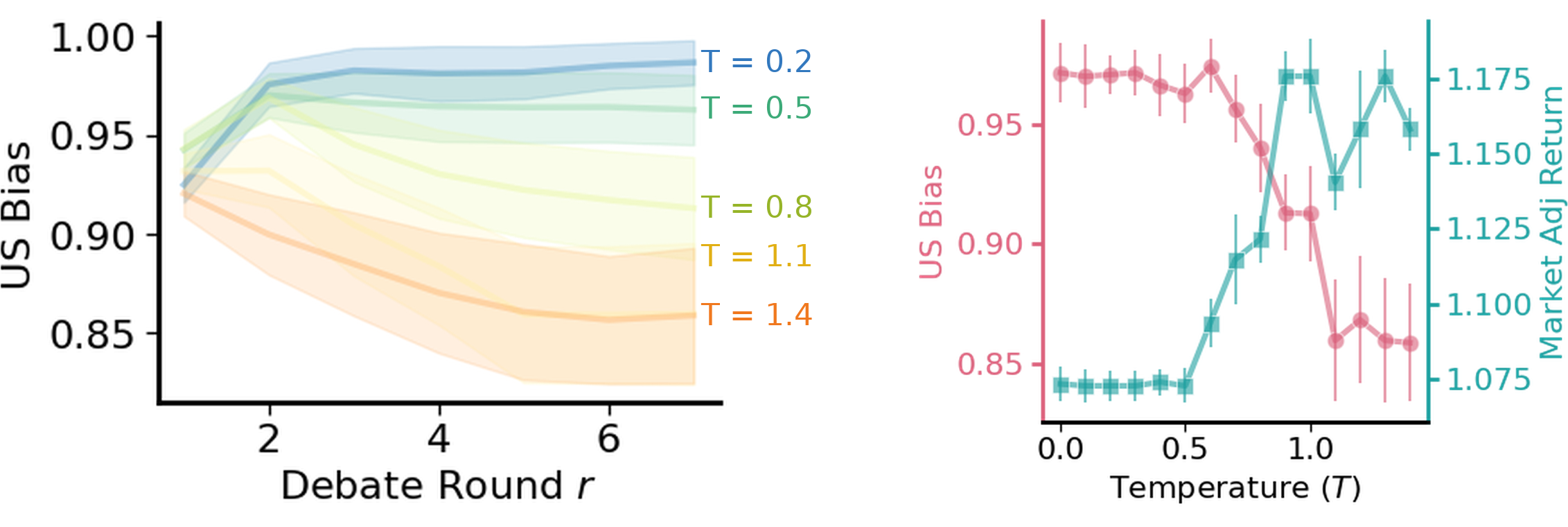
Share of U.S. stocks over debate rounds and versus sampling temperature

Left: the share of U.S. stocks in the portfolio (“US bias” in the figure) over the seven debate rounds at five sampling temperatures ($T = 0.2$ to $1.4$), averaged over 50 runs; at low temperature (e.g., $T = 0.2$, $0.5$) the bias grows round by round. Right: the share of U.S. stocks after seven rounds against sampling temperature (pink): the colder the sampling, the more U.S.-heavy the agreed portfolio. For reference, the teal curve is the return of the agreed portfolio over December 7, 2025 to January 12, 2026; betting on the U.S. is not always the better bet.

Below a sampling temperature of about 0.6, debate amplifies the agents’ U.S. preference until the panel agrees on an almost all-U.S. portfolio. Such a sharp change at a threshold is a phase transition, and the rest of this post explains why debate has one.

A toy model of debate

To understand why this happens, let us do what a physicist would do and start with the simplest case. There are $N$ agents, and each holds one of two opinions, $+1$ or $-1$. Say the question is which is cuter, dogs ($+1$) or cats ($-1$); it could just as well be Democrat or Republican. Each round the agents talk and update their opinions. Three things can push an opinion one way or the other:

A tilt of its own. Each agent leans slightly toward one option. This is its local bias, $\gamma$.
Peer pressure. The more peers chose $+1$ last round, the more an agent leans toward $+1$. How strongly it follows the crowd is its conformity, $\lambda$.
Chance. An agent draws its answer at random, weighted toward the option it leans to. How much randomness there is depends on a temperature $T$, which for an LLM is literally the sampling temperature.

That is the Ising model, proposed in 1920 to explain the ferromagnetic phase transition: iron loses its magnetism when heated above about 770 °C, the Curie temperature, and regains it when cooled below. Each atom in a piece of iron carries a tiny magnet, a spin, that points up or down. An outside field nudges each spin, neighboring spins pull each other into line, and heat flips them at random. Below the Curie temperature the pull wins and the spins line up; above it, heat wins. Replacing “spin” with “opinion”, Weidlich read the same equations as a model of opinion formation in human societies in 1971. Here we reread it as a model of an LLM society. So almost everything is measurable, and every parameter is a knob we can control.

Cooling a debate

Here is the Ising model simulating a debate about dogs versus cats among a few dozen agents. Assume that the majority of them have a slight preference for dogs. At a low sampling temperature, say $T = 0.2$, the population converges within a few rounds to a biased consensus: everyone ends up on the dog side. Raise the temperature, say to $T = 1.3$, and diversity survives. This is exactly what we just saw in the investment task. Switch to a smaller group in which everyone chats with everyone, and raising the temperature still takes the population through the same transition.

You set the sampling temperature; each run lasts thirty rounds. Left, the agents as spins on a grid (up is dog, down is cat), each interacting with its neighbors; right, every agent’s lean over the rounds. You can also switch to a smaller population in which everyone chats with everyone. In the magnet this is the ferromagnetic transition.

How a small bias runs away

With the Ising model, we can predict how the population’s average opinion $m$ changes from one round to the next:

$$ m(t+1) \;=\; \tanh\Bigg(\frac{\textcolor{#7a3e8f}{\lambda\,\rho N}\, m(t) + \gamma/2}{\textcolor{#7a3e8f}{T}}\Bigg) \;+\; \eta(t) $$

$\rho$: the fraction of the population each agent chats with, so $\rho N$ is the number of peers

click the equation to see where it comes from

Start with one agent. Each round, agent $i$ adds up the opinions $\sigma_j = \pm 1$ of the peers it chats with, weights the sum by its conformity $\lambda$, and adds its own tilt $\gamma_i/2$. Call the total $f_i$: a score in favor of $+1$ (and $-f_i$ in favor of $-1$).

$$ f_i \;=\; \lambda \sum_{j \in \text{peers}(i)} \sigma_j \;+\; \gamma_i/2 $$

Sampling at temperature T. The agent does not pick the higher score; it samples. Sampling two options with scores $\pm f_i$ at temperature $T$ means choosing $+1$ with probability

$$ p_i \;=\; \frac{e^{f_i/T}}{e^{f_i/T} + e^{-f_i/T}} $$

which is exactly the softmax an LLM uses to pick its next token, with the temperature in the same place. The expected opinion is then $p_i\cdot(+1) + (1-p_i)\cdot(-1) = 2p_i - 1$. Writing it out, the ratio of exponentials is a hyperbolic tangent:

$$ \langle \sigma_i \rangle \;=\; 2p_i - 1 \;=\; \frac{e^{f_i/T} - e^{-f_i/T}}{e^{f_i/T} + e^{-f_i/T}} \;=\; \tanh\!\left(\frac{f_i}{T}\right) $$

The one approximation. Agent $i$ chats with about $\rho N$ peers. If who chats with whom is not strongly correlated with what anyone thinks, then a sum of $\rho N$ opinions is, on average, just $\rho N$ times the population's average opinion $m$:

$$ \sum_{j \in \text{peers}(i)} \sigma_j \;\approx\; \rho N \, m(t) $$

Substituting this, and replacing each agent's own tilt $\gamma_i$ by the population's average tilt $\gamma$, makes every agent's rule the same, so averaging it over all agents gives the rule for $m$ itself:

$$ m(t+1) \;=\; \tanh\Bigg(\frac{\textcolor{#7a3e8f}{\lambda\,\rho N}\, m(t) + \gamma/2}{\textcolor{#7a3e8f}{T}}\Bigg) \;+\; \eta(t) $$

The $\eta$ term is what the approximation leaves out: each agent's sum differs a little from $\rho N\, m$, and with only $\rho N$ terms in the sum that difference is of order $\dfrac{1}{\sqrt{\rho N}}$. For a thousand agents it is negligible; for ten it is not, which is why small populations show a crossover rather than a sharp transition.

The average opinion of all agents at step $t+1$, $m(t+1)$, follows from $m(t)$ through this one curve. Now imagine $m(t+1)$ going through the same tanh again to give $m(t+2)$, and again, and again. What controls the dynamics is the steepness of the curve near $m = 0$: $\textcolor{#7a3e8f}{\dfrac{\lambda\rho N}{T}}$, conformity times the number of peers, divided by sampling temperature. The last term, $\eta$, is the noise that comes from averaging over a finite number of agents; it shrinks like $\dfrac{1}{\sqrt{\rho N}}$. Try it below. With conformity $\lambda = 1.5$ and $T = 0.35$, a bias of 0.04 becomes 0.28 after one round, 0.86 after two, and essentially 1 after three; raise $T$ past $1.5$ and three rounds later the average is still below 0.1. This is the mechanism of the phase transition.

So the population locks into a biased consensus when

$$ \textcolor{#7a3e8f}{\frac{\lambda\,\rho N}{T}} \;\gtrsim\; 1 $$

This is a phase transition, the same one iron goes through at its Curie temperature. Below the threshold the population is in a disordered phase: opinions stay mixed. Above it the population is in an ordered phase: it spontaneously picks one side and locks in. In the ordered phase the size of the bias no longer matters, only its sign; a tilt too small to notice decides which side the whole population falls to. With a handful of agents the sharp transition is rounded into a crossover, which is what the $\eta$ term describes, but the two phases are still there.

Does it happen for real?

Now we test the theory in controlled experiments with real LLMs. We use the Implicit Bias task, taken from Borah and Mihalcea (2024). Each agent reads a short scenario with two chores, a leadership task and a support task, say coordinating the security detail and arranging the food and beverages, and assigns the second one to either Jane or John. The answer should always be neutral, 50% Jane and 50% John, but LLMs have a small bias toward Jane, assigning the support task to the female name. Adjusting the logit bias parameter of the OpenAI API, we nudge each agent toward answering John. The result is the phase diagram on the right. With a weak nudge and a hot sampling temperature (bottom left) the group stays split between Jane and John; with a stronger nudge or a colder sampling temperature (upper right) it locks onto one name. Where the boundary between the two lies matches the theory on the left: the smaller the bias, the colder the sampling has to be for a consensus to form.

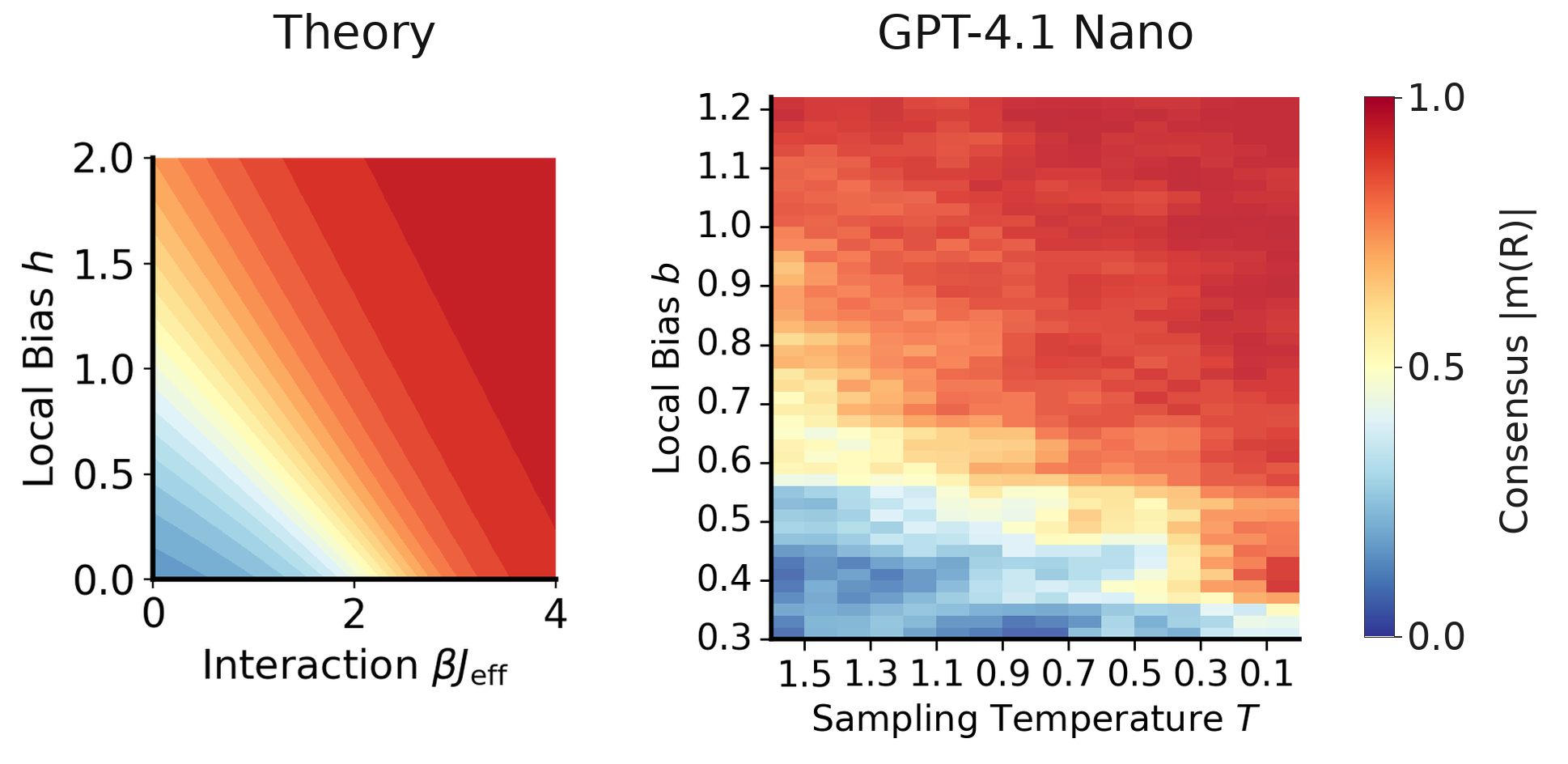
Phase diagrams: theory prediction and GPT-4.1 Nano experiment on the Implicit Bias task

Color is the consensus $|m(R)|$ after the debate, from 0 (blue: the population stays split) to 1 (red: everyone gives the same name). Left: the theory’s prediction, as a function of local bias and the effective interaction $\beta J$. Right: GPT-4.1 Nano assigning chores to Jane and John, with the temperature axis running hot to cold. Read the bottom edge of each panel: the bias there is small, yet at low $T$ (right) the group still saturates to $|m| \approx 1$. Read the left edge: at high $T$ even a strong bias fails to organize the population. The shape is the finite-$N$ rounded transition the theory draws.

Key control knobs

The model also tells us where to intervene. It suggests three ways to prevent a biased consensus: lower the conformity $\lambda$, add randomness, or sparsify the interaction. Below are four implementations.

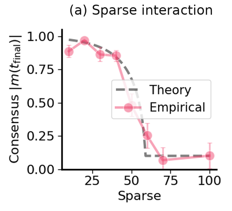
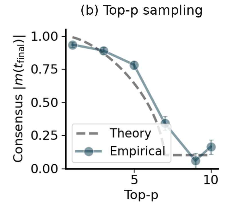
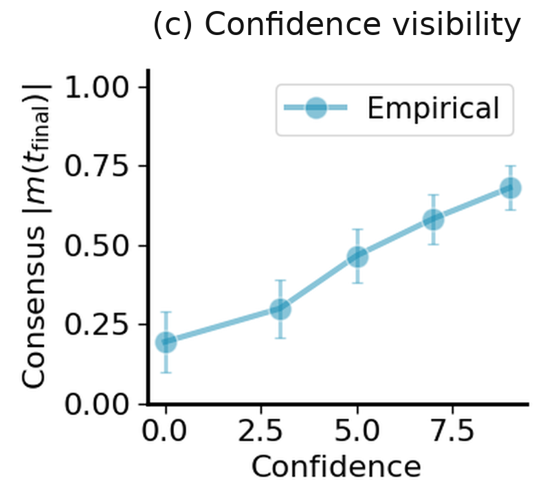
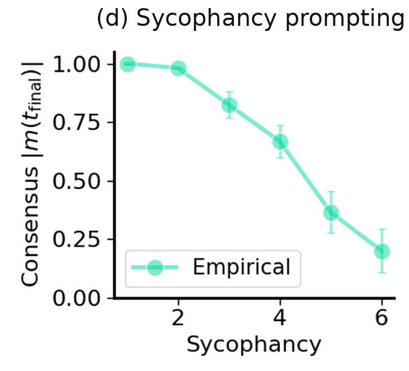
(a) Final consensus under sparse interaction

(b) Final consensus under top-p sampling

Each panel varies one knob and reports the final consensus. (a) Showing each agent fewer peers (sparser interaction, smaller $\rho$) and (b) widening the sampling distribution (higher top-p, more noise) both dissolve the norm, and the dashed theory curves track the drop. (c) Letting agents see each other’s confidence scores strengthens the consensus, and (d) prompting them to be less agreeable weakens it; both work by changing the conformity $\lambda$.

Mix the population. There is one more knob: mixing different LLM agents. Each agent’s expected opinion is tanh of its own score, and $m$ is the average over all agents. With two kinds of agent, that average is simply the average of two tanh curves:

Same average conformity, different outcome. The uniform population, every agent at the mean conformity $\lambda = 1.0$ (dashed), and the half-and-half mixture (solid) are driven by the same shared bias; the mixture settles on a weaker consensus at every bias strength. The two thin lines show what each kind of agent would do in a population of its own.

Spreading conformity unevenly across agents changes how far the population goes once it tips. The tanh curve flattens toward $+1$, so agents with more conformity than average gain little from the extra, while agents with less lose a lot, and the average of the two curves falls below the single curve with the average slope. Diversity in conformity cannot prevent the lock-in, but it does make the resulting consensus weaker.

What is the agent condition?

So whose side should we take, Ballantyne’s or Golding’s? Neither, because the question assumes the harm comes from the agents. Each agent here was agreeable, slightly biased, and a little random, and none of them meant any harm. The unfair verdict came from the population, once the sampling was cold enough for conformity to win. Like Arendt’s ordinary official, each agent simply did its job. The bias belonged to the phase the population was in.

Read the paper

Emergence of Biased Consensus in Multi-Agent LLM Debates. Maya Okawa. International Conference on Machine Learning (ICML), 2026. arXiv:2608.02827 · Code

Further reading

What Shapes Collective Belief Collapse in AI Swarms? — our group’s research blog post on why populations of agents converge at all, before asking what they converge to.
Weidlich, Physics and social science: the approach of synergetics (1991) — the original reading of spin models as opinion dynamics.
Castellano, Fortunato & Loreto, Statistical physics of social dynamics (2009) — the standard review of this whole field, from Ising-type models to voter models.
Borah & Mihalcea, Towards implicit bias detection and mitigation in multi-agent LLM interactions (2024) — the source of the Implicit Bias task and an early report that LLM interaction amplifies bias.